Timbral Evolution: Harmonic analysis of classic synth sounds

This post is a place to gather my thoughts about one of the most important parts of synthesizer design: the timbral evolution of sounds. It also presents the results of my analyses of some classic synth sounds.

There have been many methods developed over the years to achieve timbral evolution. The voltage-controlled filter is the first and most obvious. Pulse width modulation and oscillator synchronization are two more from the analogue era. Other later approaches include wavetables, vector synthesis, FM, phase distortion, and others.

The aim of all of these concepts is the same; to provide timbral evolution during the course of a sound. I would argue that many sounds have a richness and interest to the human ear because of the non-linear changes in their harmonic structures over time. Effective and efficient generation of these interesting non-linear changes is a fundamental challenge that synth designers must meet if their instruments are to make sounds that grab you.

Pulse Width Modulation

Pulse width modulation is one of the classic synth sounds, and provides a level of depth and richness that is otherwise hard to achieve on an analogue synth. The only other common analogue technique with similar power is oscillator synchronization, which we’ll look at shortly.

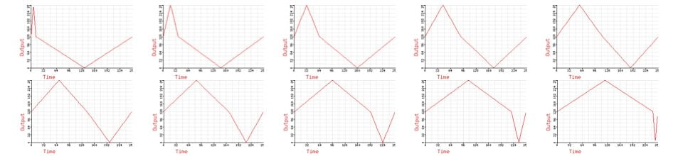
These nine graphics show the changing shape of a pulse wave as the duty cycle (the ratio of high to low time) is altered between 10% and 50%. These pulse waves were generated using additive synthesis of the first 100 harmonics. The relative levels of the harmonics in the pulse wave are given by the following formula:

Harmonic Amount = sin($h  * Pi * $d) * (2 * $a) / ($h * Pi)

$h is the harmonic number, $d is the duty cycle (0-1) and $a is the amplitude.

In addition, the waveform has a DC component:

DC component = $duty_cycle * $amplitude

Note that these equations generate a unipolar pulse wave.

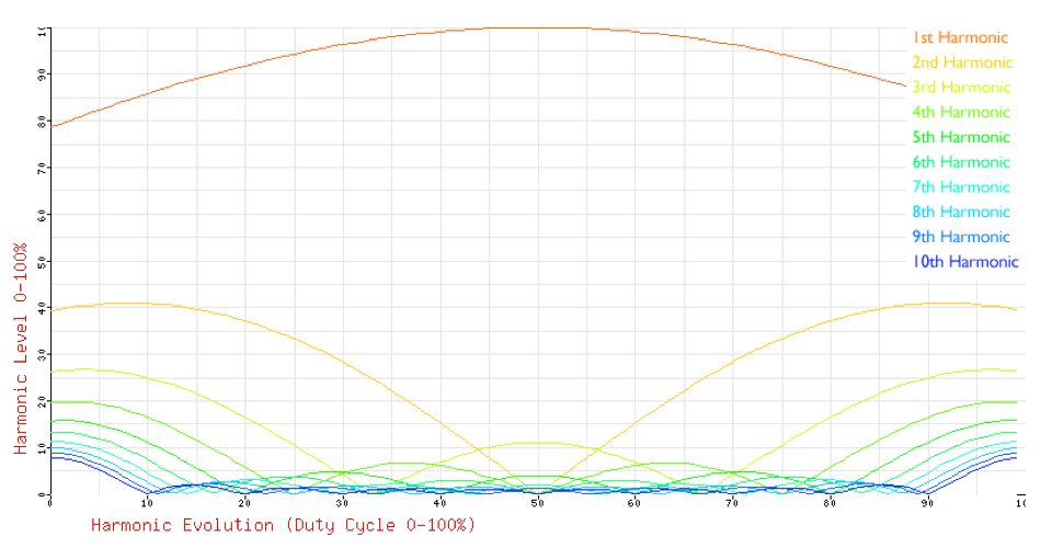
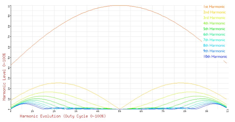
The important thing about this for the synthesist or synth designer is that the harmonic spectrum changes in a nonlinear, complex way when the duty cycle is altered. We can plot the harmonic variations:

The graph shows the way the amount of the first 10 harmonics alters with varying duty cycle. Since the second half of the graph is a mirror image of the first, many synths have pulse width controls that run from 0% to 50%, rather than all the way to 100%.

In the same way that a static spectrum graph describes the sound of a ramp wave, this graph describes the sound of PWM.

Phase-shifted waveforms

Another classic analogue sound is the effect of two oscillators detuned against each other. This produces a changing phase-shift between the two signals. This phase-shift cancels some harmonics and reinforces others.

Sum of phase-shifted waveforms

In general, when summing identical waveforms, the first harmonic will decrease towards zero as the phase shift approaches 180º. The second harmonic will do the same thing as the phase shift approaches 90º. The third, towards 60º. Subsequent harmonics behave similarly, with the first zero point for harmonic $h being 180º/$h. The graph below shows this behaviour:

The level of a given harmonic $h at a phase shift of $phase degrees is given by:

Harmonic Amount = abs( cos( Pi * $phase/360 * $h ))

A harmonic obviously cannot be cancelled from a waveform unless it is present to begin with, so the harmonic amount above must be multiplied by the level of the harmonic in the original waveform that we are phase-shifting. To take a simple example, a ramp wave includes the third harmonic at a level of 1/3, so the level of the third harmonic in the sum of phase-shifted ramp waves is:

Harmonic Amount = 1/3 * abs( cos( Pi * $phase/360 * $h ))

Note that we are ignoring the phase of each harmonic here, or assuming that it zero.

Difference of phase-shifted waveforms

If instead of summing the waveforms, we take the difference, the two signals start out completely cancelled. In this case, the first harmonic increases towards the maximum level as the phase shift approaches 180º. Likewise, the second harmonic increases to maximum as the phase shift approaches 90º. This produces a graph closely related to the one above:

The level of a given harmonic $h at a phase shift of $phase degrees in this case is given by:

Harmonic Amount = abs( sin( Pi * $phase/360 * $h ))

Again, for any particular source waveform, this harmonic amount must be multiplied by the level of the harmonic in the source waveform. Using our previous example, a ramp wave includes the third harmonic at a level of 1/3, so the level of the third harmonic in the difference of phase-shifted ramp waves is:

Harmonic Amount = 1/3 * abs( sin( Pi * $phase/360 * $h ))

PWM as a special case of phase-shifted waves

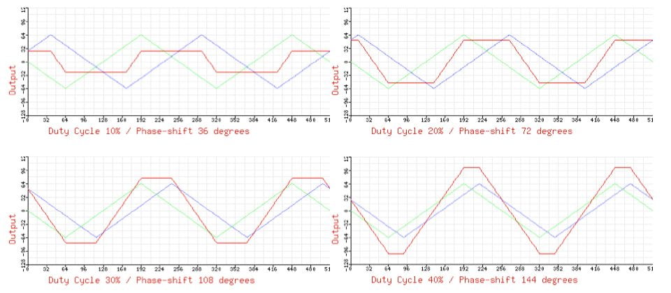
One way of generating pulse-width modulated pulse waves is to take the difference of two phase-shifted ramp waves. Equivalently, you can sum a ramp wave and an inverted ramp wave. The images below show various duty cycles (in red) created by summing the blue and green ramp waves.

We already know that the level of a given harmonic in the difference of phase-shifted ramp waves is:This demonstrates the equivalence of PWM to the difference of phase-shifted ramp waves. If the harmonic levels for the harmonic evolution on the previous page are scaled to the levels present in a ramp wave, the result is the harmonic evolution for PWM that we’ve already seen.

Harmonic Amount = 1/$h * abs( sin( Pi * $phase/360 * $h ))

This seems to produce pulse waves, so this equation must be equivalent to the one we saw earlier for pulse wave harmonics:

Harmonic Amount = sin($h  * Pi * $d) * (2 * $a) / ($h * Pi)

$h is the harmonic number, $d is the duty cycle (0-1) and $a is the amplitude.

Note: The 2*$a/Pi term is a simple adjustment for the summed amplitude. But the equation I’ve got doesn’t include phase, which obviously varies. I know this is significant for my pulse waves since I had to use cosines to sum together to make a successful pulse wave.

This means that rather than being a special case, pulse width modulation is actually just one case of a whole general category of harmonic evolutions generated by phase-shifted waves. By changing the source wave, and whether the sum or difference is used, many other related harmonic evolutions can be generated.

Another example is shown below; a double-pulse wave, created from the sum of phase-shifted square waves. Varying the phase shift in this case produces a symmetrical pulse width modulation of both positive and negative pulses.

Another example is

Oscillator Sync

We can do a timbral evolution analysis for oscillator synchronization in exactly the same way that we did for PWM. This will give us the specific sonic fingerprint of those amazing “sync bend” sounds. Unlike PWM which is limited to duty cycles between 0% and 100%, oscillator sync has no ‘upper limit’ for the ratio of the slave frequency to the master frequency. The waveforms and analysis below show the effect up to a slave/master ratio of 3.5.

The graph was generated by Fourier analysis of naive ramp oscillator sync waveforms. The points where the waveform becomes a simple ramp at twice and three times the master frequency are clearly visible (sync ratio = 2.0, sync ratio = 3.0).

Phase Distortion

Another technique which can produce non-linear changes in the harmonic spectrum is phase distortion (PD). If you don’t understand how phase distortion works, there’s a page about it elsewhere on the site.

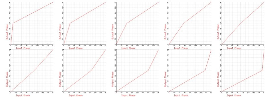
One easily-produced phase distortion function is the ‘knee function’. Changing the distortion index changes the shape of the function and hence the resulting sound. Example knee functions for various indices are shown below:

Ramp-down/Triangle/Ramp-up

The output from this knee function will depend on the source waveform that is fed into it as well as the degree of distortion, and many of these transformations would be impossible to reproduce with analogue electronics.

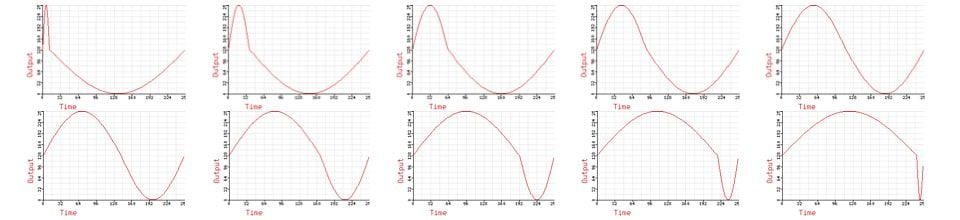
One transformation produced by the knee function that you can do with analogue electronics is the ramp-down/triangle/ramp-up:

The harmonic development of this waveform is show below. Note the moment at 50% where the waveform becomes a triangle, and all the even harmonics become zero.

Sine Wave

This same phase distortion knee function can be applied to a sine wave. The resulting waveforms are shown below:

The harmonic evolution of this waveform is similar to the triangle wave case. This is probably to be expected as the triangle wave is not a million miles from the sinewave.

The effect of source waveform phase on phase distortion

It should be noted that the phase of the source waveform is important.

Phase-shifted triangle

If we apply the knee function to a a triangle wave that starts at the centre value rather than the lowest value, we get completely different waveforms.

The harmonic evolution of this is also different, and even closer to the sine wave case we’ve just seen:

Cosine Wave

Likewise, if we apply the knee function to a cosine wave rather than a sine wave, we get a waveform that approaches a ramp at the extremes. This almost-ramp waveform appeared in the Casio CZ phase distortion synthesizers.

There are many other phase distortion algorithms possible, and they will have their own characteristic harmonic evolution.The knee function can also be applied to a square wave, in which case it produces PWM, which we’ve already looked at.

Frequency Modulation

The timbre in FM synthesis depends on the ratio of the modulator to the carrier and on the modulation index, the depth of the modulation. Although ratio affects the frequencies of the sidebands (and hence the timbre), it does not affect their amplitude. The sideband amplitude is determined entirely by Bessel functions of the first kind. The way the Bessel functions change with changing modulation index defines the “FM sound”.