
I’ve been curious about Chorus for a while, since I’ve been working on and off with chorus design myself. There were a few things I didn’t understand, like what the relationshp is between the modulation LFO’s waveshape and the frequency modulation of signals going through the chorus. You’d think that if you use a sinewave to modulate the BBD clock, you’d get a sinewave modulation of frequency, right? Wrong! So what do you get? At this point, I realised that it was a bit more complicated than I was giving it credit for and I’d have to really think about it. This page is some of the results of those studies.
Simulation of BBD chorus
So what did I do? Well, I did what I always do when I don’t understand something. I wrote a simulation of it. If I can write a sim of a situation, then I know that I understand it. If the sim doesn’t work, there’s something I’m still missing. Often the process of thinking about how to simulate something, and seeing how and why the simulation doesn’t work gives me an insight into the real situation. If that doesn’t work, playing with the simulation gives me a useful way to perform repeatable experiments that would often be awkward to do in reality.
My simulated delayline has 1024 stages, just like the SAD1024, MN3007, or MN3207 chip. Of these, only the last one is still available, so it’s the chip likely to turn up in modern analog chorus designs.
My chorus has linear clock modulation like the typical chorus effects. More about the problems this causes later – for now, we’re just simulating a typical chorus. The clock frequency at any given moment is:
$clock_freq = $clock_centre_freq + ($lfo * $mod_depth * 10000); // 10KHz mod range
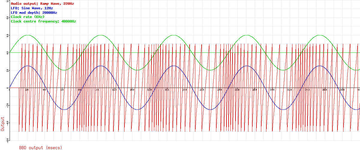
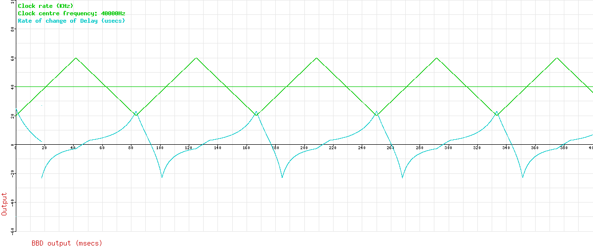
Here’s the LFO waveform (blue) and the Clock rate (green). The horizontal green line is the clock centre frequency with no modulation applied. You can see that with a modulation depth of 20KHz, the clock frequency goes up to 60KHz, and down to 20KHz. The LFO rate and Clock rate are just chosen to give a reasonable display. We can see 400msecs of signal here.

Ok, so far, so good. Let’s feed some audio into it and see if we can see anything happening. Remember this is just the signal through the BBD (the “Wet only” signal), so it’s not a full chorus. In fact, it’s just a vibrato unit. But mixing the dry and wet signals together is easy, and that’s not the bit I don’t understand, so I’m ignoring the dry signal. This next graph adds a low audio ramp wave (red). You can easily see the pitch change caused by the clock modulation. Notice the initial delay before any signal comes through the delay line is clearly visible on the left hand side of the graph.
Now this is where things start to get interesting. What do you think is happening to that audio frequency? It should be varying up and down, following the changes in the clock rate, right? Let’s have a look. The next graph uses the slope of the output ramp wave to give an estimate of the audio output frequency at each moment. This is only possible with ramp waves of fixed amplitude, but it’s handy for our demo. This is plotted in red. I’ve taken the LFO off to stop it getting too cluttered.
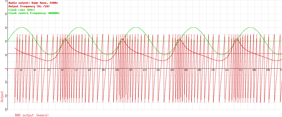
Interesting, don’t you think? The frequency modulation produced isn’t a simple sine wave – it’s distorted. Let’s have better look at that without the audio:
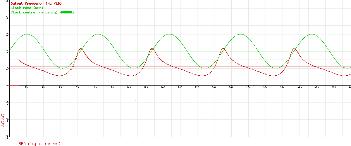
So what’s going on here? Think about how the BBD makes a pitch change. When the LFO output is rising, the clock frequency is increasing, and samples are being read out faster than they were read in – their pitch is shifted up. Likewise, when the LFO is falling, the clock frequency is decreasing, and samples are read out more slowly than they were read in – the pitch is decreased. The key here is that the pitch shift is not caused by a high clock frequency or a low clock frequency, but by an increasing or decreasing clock frequency. It’s the rate–of–change of clock frequency that’s important.
For a sine wave LFO input like we’ve been using, the point of maximum increase is the middle of the upwards slope, where our clock rate crosses the horizontal red line. Similarly, the maximum decrease is on the downwards slope where it crosses the red line. If we plot this rate of increase, we’re plotting the differential of sin(x), which is just cos(x) – the same thing shifted forwards a bit.
But hang on a minute! Our frequency modulation isn’t following cos(x) for our sin(x) LFO! That curve isn’t a cosine curve any more than it’s a sine curve. Where’s that distortion coming from?
Why does the modulation get distorted?
Let’s back up for a moment and consider the delay. How would we measure the delay at any moment in time? Well, the total amount of delay is just the amount of delay provided by each bucket, all added together, and how much delay you get depends on how fast the clock was going for each of the previous buckets. The delay for a single bucket is the length of time since the last clock pulse – e.g. the clock period. The total delay is the sum of all the last X clock periods, where X is the number of BBD stages. Put another way, we’re integrating the area under the clock period curve for the last X samples.
Let’s plot the clock period curve. Here it is, added to the graph in green:
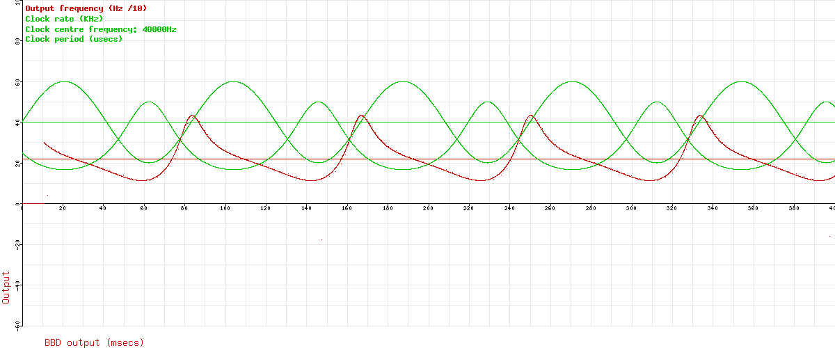
The first thing to notice about this is that it’s already slightly distorted, since we’re now looking at 1/sin(x) rather than sin(x). But the distortion is all in the vertical direction, not in the time axis. To say that another way, the waveform is still symmetrical left-to-right. Ok, now let’s see what shape curve the delay makes if we add up the last X periods of that clock period graph. Here it is in blue:

Now we see where the rest of the distortion comes from. Although the clock frequency matches the LFO, the actual delay doesn’t directly, because it is the sum of all the clock periods for the whole length of the delay line. Incidentally, with the clock frequency we choose originally, the blue line goes from slightly below 10msecs to slighty above 20msecs, so we’re pretty much in chorus territory here.
But it still doesn’t look like the frequency modulation!
Well, no, true. It doesn’t. But you remember when we talked about it being the rate-of-change of delay that was important? We were thinking that for a sin(x) LFO, we’d see a cos(x) frequency modulation? It isn’t that simple, since as we’ve shown, the total delay follows a much more complicated curve than the clock frequency. But the point still stands – it’s the rate-of-change of delay that matters. Here’s the plot with the rate-of-change added in pale blue:

Now at last we’ve got a waveform that looks like our frequency modulation! The frequency modulation follows the rate-of-change of the total delay, and that waveform isn’t anything like the modulation LFO’s waveform.
Great! So what frequency modulation do I get with other LFO waveforms?
Ok, let’s have a look at a few in isolation. First we’ve got the sine wave LFO that we’ve just seen:

A triangle wave LFO is probably even more common, since they’re easy to build:
And square wave LFOs are even easier to build, but rarely used for chorus:
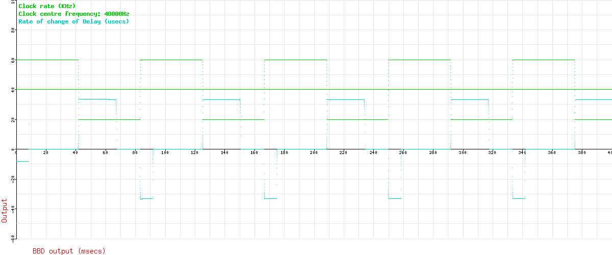
Now, there’s an interesting result! Although the LFO jumps between two levels, the output frequency jumps between three!
Linear versus Exponential clock modulation for BBD chorus
One of the problems with a typical chorus unit is the pitch modulation gets deeper as the BBD clock rate is reduced (e.g. as the delay is made longer). This makes the pitch variation very obvious – “seasick” or “warbley” are words often used to describe the sound. A typical chorus unit uses an LFO to modify its clock frequency, and that clock modulation is linear, so a given modulation depth will give (for example) +/-25KHz of clock modulation. This is how our simulation has operated thus far. When I considered this, it seemed to me that must be the reason why the depth seems to go up. If you consider a high clock frequency of 200KHz, a modulation of +/-25KHz is about 12%, or about 2 semitones. If you then consider what happens at a low clock frequency of 50KHz, the same modulation of +/-25KHz now shifts the clock by about 50%, or roughly an octave (50-25 = 25, which is 50% of 50KHz, 50+25 = 75, which is 150% of 50KHz).
So what’s the solution? Use exponential frequency modulation like a synth VCO of course! Then the LFO mod depth would be specified as “an octave” or “4 semitones” and an octave shift at 50KHz is the same as an octave shift at 200KHz.
An Update – some further thoughts
A while after posting this article, I had an email discussion about it with Brian Neunaber of Neunaber Audio Effects. Brian was initially slightly sceptical about the effect I claimed to have found and thought it might be an effect of the simulation or the frequency measurement method. This challenge pushed me to ensure that the method and results were sound. Once I’d convinced him that the effect was real, he wrote out the equations for what I’ve stated above and modelled them in Wolfram Alpha. I’ll reproduce his working below.
Firstly, we know that the total delay is related to the number of stages and the clock frequency:
total_delay = 1024 / (2 * clock_freq)
Note that clock_freq doesn’t have to be a constant. It could vary.
We also know that the change in pitch is related to the rate-of-change of the total delay:
change_in_pitch = d/dt (1024 / (2*clock_freq) )
Now, how about we make our clock have a base frequency of 40KHz, and modulate by +/-20KHz:
clock_freq = (40000 + 20000 * sin(2*pi*2*t) )
Put that into the pitch change equation:
change in pitch = d/dt (1024 / (2 * (40000 + 20000 * sin(2*pi*2*t) ) ) )
We can plot that in Wolfram Alpha. This shows us our by-now-familiar distorted curve. Brian wondered how much actual pitch change that represents, so he also plotted log2(1+x) in Wolfram Alpha to see how much shift in octaves that is. The maximum pitch change is around 0.2 octaves, or approximately 2.4 semitones. That’s quite a lot for a chorus, and another plot shows that if we reduce the modulation depth, the distortion also decreases. It seems reasonable to me to suspect that slower LFO rates also decrease the distortion, since it usually reduces the waveform’s rate of change (though not for a sharp square wave). On this basis, the effect won’t show up on slow, shallow chorus waveforms like I initially thought, but will definitely be present on deep, fast flangers. Perhaps this article should have been titled “Investigations into what a BBD Flanger unit *really* does” instead!
My thanks to Brian for the discussion and his thoughts on the matter.
Study the ARP Omni service manual on its ensemble generator. It also uses expo modulation.
Thanks for the tip! I shall look it up.
Nice work. Though the optimum frequency modulation for chorus is not exponential. It is hyperbolic, as that gives zero pitch warble. For small modulations, an exponential modulation looks approximately hyperbolic which is why it works OK.
Something I noticed when analyzing the Boss CE-2 is that the clock frequency modulation counter-acts the frequency modulation effect on delay time. For the total frequency deviation in that circuit (about 8.5ms to 10.75ms) the final delay change function is a slightly “swollen” triangle wave when fed with a triangle oscillator.
Here’s the clock frequency function:
vf : Final voltage, or where clock input chip tips over (GND – 1V, which in this circuit “GND” is 9V, so this is 8V)
vi: Initial voltage as set by the buffer transistor from the LFO. This is where the oscillator starts after reset.
va: Applied voltage (switched to 9V when charging).
tau: R*C, in CE-2 this is 150k * 47p
ts: Switching period
fs: Switching frequency
trst: reset time
ts=-tau*ln( 1 – (vf-vi)./(va-vi) )
fs=1./(ts+trst)
Delay = N_STAGES/(2*fs)
If you plot delay time vs LFO voltage you end up with something that looks like a mildly (1-e^x) type of shape, when evaluating the max error from a linear interpolation from max delay time to min delay time the straight line was no more than 1% error.
That said, it would appear from the CE-2 and variants using the same type of LFO control, this is a linear transfer from LFO to delay time within 1% error.
Now triangle delay shape to pitch is as you pointed out.
In this case the mild exponential distortion makes for a less abrupt pitch change at the LFO peaks.
Furthermore, there is a flattening of the LFO bottom at more extreme depth settings, which limits the lower clock frequency in an asymmetrical way. In other words, this gets more interesting at the lower end of the LFO sweep due to the series diode drops and effect of them turning on.
Hi Tom,
Love your stuff, this article is particularly interesting.
The wave shape used for modulating the legendary Roland Dimension D chorus is something like a soft clipped sine. The native chorus plugin for Logic Pro X uses something similar. I think this may be what DrAlx referred to as hyperbolic. TanH possibly.
Your TapLFO has a waveform based on sine+3rd. I noticed while playing around with this additive waveform generator… https://meettechniek.info/additional/additive-synthesis.html that adding in the 3rd harmonic with an amplitude of about 10-12% produces something very similar to a TanH waveform.
Is it possible for the user to modify your TapLFO wave table?
Yes, it’s possible. If you look at the code, you’ll find the sine waveform table at the bottom. You’d have to generate new data using whatever your favourite tool is (I use a PHP script, but anything will work). Then paste it in, and rebuild and program it to a chip from MPLAB X.
Thanks Tom
Interesting article.
If it’s of any value, I used to mess around with BBD devices (before digital became a realistic alternative for home constructors) and this ‘non-linear’ pitch shifting was annoyingly evident when modulating a linear VCO clock source with triangular or sinusoidal waveforms.
I never tried to mathematically unravel it but my thinking was that there were two effects going on. One, as you state, the amount of pitch shift is related to the rate of change of the delay time and the second is that the longer the delay time the greater the pitch shifting effect, but this is also a function of the relationship between the delay time and the wavelength of the signal passing through. If the delay time is much shorter than the wavelength, the amount of pitch shift with a given modulation rate will be smaller than with a longer delay or shorter wavelength.
As a result the modulation waveform’s effect on pitch shift varies over its cycle and the change of polarity at the longest delay is most pronounced. I read somewhere (possibly an E&MM magazine) that this effect can be compensated for by changing the shape of the mod waveform. A triangle waveform was suitably biased and put through a diode to perform a logarithmic conversion of sorts, to produce a very nonlinear asymmetrical waveform with a sharpish peak and shallow bottom. I seem to remember that this worked quite well but took a bit of fiddling with levels and bias to get an optimum waveform. But every time you changed the delay time, the depth of modulation had to be adjusted to get the effect right. Room for improvement…
Thanks for your comments. I’ve seen several analog effects that use the so-called “hypertriangular” waveform, which is a triangle wave with the bottom points rounded off. I included a “Sweep” wave in several of my LFO design which provides something similar (my Sweep wave is the lower half of a sine, but it’s at least as close as the distorted-triangle analog original. For the Flangelicious, I included exponential control of the clock which helps linearise things, but isn’t the whole story.
It’s a lot more complicated than most people give it credit for!!
I kind of wish I hadn’t read this article now. It’s got me thinking and until I understand this apparently straightforward system, it will bother me a little. I don’t have the means to simulate so I am somewhat limited in quantifying the ideas that I will attempt to express.
I started out by considering the two extreme cases of modulated delay line systems, one with a delay time of zero and the other with a delay time of infinity. In the first case, no amount of modulation will affect the signal passing through since the input and output sample periods for a given sample are essentially the same. In the latter case anything that happens at the input is so far behind what is happening at the output it can be ignored. The sample rate and variation thereof essentially only affect the output. In this case the frequency shift of any signal held in the delay line is directly proportional to the sample frequency. But in reality (and more usefully), we have something in between where the delay line time is not so far from the modulation waveform period. They interact and this where the strangeness lies.
I have re-read and think I understand everything that you have said and it all makes sense. The final square-wave modulation plot nicely illustrates the angle that I am coming from on this and is to be expected. If you have a continuous tone passing through the delay line and you step change the sample frequency, say upwards; the output tone pitch will step change upwards proportionally but at the same time the input sample rate has increased. After the delay line time at this higher sample frequency has elapsed the input samples taken at the higher sample rate have shifted through to the output and the output tone pitch will shift back to where it was… the steady-state condition. If the sample frequency now step changes to a lower value, the output tone pitch will drop proportionately as the samples are now read out at a lower rate and the input samples are now read in at a lower rate. After the delay line time (at this longer delay) has elapsed, the input samples at the lower sample rate will have shifted through and again the tone will return to its steady-state value.
It is easy to predict the effects of a square-wave modulation when the modulation period is much longer than the longest delay time but where it gets confusing for me is when the modulating waveform is continuous. At any given moment, although the input and output sample rates are always the same, by the (continuously variable) time the input samples are clocked through to the output, they are clocked out at a different rate. The effect of this is not so easy to predict with mere grey-matter.
30 odd years ago I modified an Ibanez digital delay pedal that had a maximum delay time of 1800mS. I disconnected the on-board clock source and connected cables so that I could provide my own modulated clock. I seem to remember that the smoothest and lushest chorus effects could be obtained with long (echo territory) delay settings but as a consequence you had a full level echo thrown in for free. Not always useful… Shortening the delay time to normal chorus territory resulted in the difficulties described at the beginning of this article.
Can’t put this one to bed until I understand it!
I set up an Excel spreadsheet to simulate some of what I think is going on and the results seem to support my thinking… I’ll try to keep this brief.
In order to take into account the changing delay line time with respect to the clock modulation signal I generated the sample periods for 1024 consecutive samples (each one needed the previous one to be calculated first) and then look at the ratio between the first and last sample periods to give me an indication of the pitch shift. I use a macro to repeatedly plug in the clock frequency at regular phase angles of the modulating signal at the beginning of the 1024 calculations and plot the sample time ratio against modulation phase angle. This is a brute force and workaround approach and I’m not actually modelling a signal passing through the system but I think it is valid… the results with simple, known scenarios certainly concur with what is understood, but other results (if correct) show very non-linear behaviour and interrelations.
I only use a sinusoidal modulating source. I can enter its depth and frequency and the clock offset frequency.
It seems the depth of modulation (w.r.t clock frequency) “distorts” the shape of the “pitch shifting” even with low modulation frequencies. When the depth is kept constant, if the modulation period is equal to the offset delay time there is no pitch shifting and the same applies to multiples of the modulation frequency. Maximum “pitch shifting” occurs between these multiples and when the modulation period is twice the offset delay time. Modulation frequencies below this seem to have progressively less effect.
I could develop the spreadsheet further to get more comprehensive results more elegantly but I thought I would just throw it out there for consideration and criticism.
I think you raise a good point mentioning the delay time. The delay times are frequently “short” compared to the LFO period – say 5-20 msec delay versus 100 msecs to 10 secs LFO period.
You’ve spotted that if the delay time is the same as the LFO period (or a multiple of it) then the speed the samples get read out at will coincidentally be exactly the same as the speed they were read in at, and consequently there’ll be no overall pitch shift. Despite them potentially having been sped up and slowed down several times on their journey from one end to the other! Ultimately what happens “in-between” isn’t important. Perhaps that offers us another way to analyse the problem.
Thanks for your thoughts and insights
Edit: Incidentally, it doesn’t work the other way around – if the LFO period is a multiple of the delay time, that doesn’t help.
P.S. It was found that progressively reducing the depth of modulation causes the predicted pitch shift to tend towards sinusoidal.
Yes, this is intuitively what we expect, and matches my own results.
Hi Tom
Can you tell me how do you do all the simulation graphics?
which programm o code do you use?
I wrote code in PHP which generates all the graphics. There’s a simulation of the delayline, and then a graph output class which deals with all the plotting of results.
Hello from 2022! Found this page after trying to work out why my ce-2w vibrato didn’t seem to match either sine or triangle waveforms. I now understand a lot more about lfo, delay times, rate of change and resulting frequencies. Well, I thought I understood it all until that final chart with the rate of change of delay line added, seems to me that on that chart the highest (fastest?) rate of change (light blue trace) lines up with the lowest output Freq (red line), and the lowest rate (slowest change?) lines up with the highest Freq – that doesn’t make sense to me as I read the article to state the fastest rate of change should result in the highest Freq output ?
Many thanks!