Fourier Analysis for non-mathematicians

Years ago, I discovered that it was possible to analyze a waveform and discover what harmonic components it was composed of, and that the magical technique to do this was called “Fourier Analysis”. I tried to find out all I could, but all the references I could find were aimed at university level mathematicians, and I was only 12 or 13. As far as I could see, none of the books explained the technique, rather they just splurged unhelpful equations in incomprehensible notation onto the page. I was left to my own devices, and although I now realize I got pretty close, I never managed to reinvent Fourier analysis for myself.

Years later, and I learned enough to finally fathom it. When I got it, I was scandalized! Those damn cheeky mathematicians had been making out that this was somehow hard or complicated all this time, and it’s not!! I felt cheated! I decided that I needed to try and write the explanation I wish I’d had when I was younger.

This is that attempt. I like to think in diagrams, rather than equations, and if you’re of a similar turn of mind, you might find this useful. Similarly, I’m also a programmer not a mathematician, so I find code or pseudo-code an easier way to understand an algorithm than maths notation, and I’ve included PHP code for each part.

Please realize that any such explanation has to leave quite a lot of stuff out. There’s lots more to know and to understand about how the Fourier transform does the magic it does. There’s loads of stuff about all the variations (continuous time, discrete time, FFT, DFT, etc etc). My own interest is in analysis of sound waveforms, so I want to start with some sampled audio data and find out what harmonics it contains. What I’m concerned with here is simply how you get it working, and that doesn’t require much of the deeper maths (like proving the orthoganality of sine/cosine, for example – we can just use it).

Fourier Analysis without the equations

So how does it work?

Fourier Analysis is performed by multiplying the signal to be analysed with a series of sine waves. This sounds complicated, but it isn’t, because you only do one at a time, and you don’t have to do any of the others if you don’t want to. You can use the same technique to find the amount of any given single harmonic in any given waveform. You only have to do all the harmonics if you want to know the whole harmonic spectrum. If you just want the first ten harmonics, just run the algorithm ten times.

Ok, how do we do this multiplication of a sine with our signal?

The multiplication is done in the discrete time domain by multiplying each individual signal sample with the corresponding sample from the sine wave. The final result is the accumulated total of all these multiplications, the area under the curve. In continuous time, we can do this algebraically and multiply the two functions and then find the area under the curve (integration). In discrete time, a sum total of the multiplied samples stands in for this integration. This process is called “convolution”.

Let’s have a look at that step-by-step.

Convolution one step at a time

The first step is the multiplication of a signal sample with the corresponding test sine wave sample. This is shown on the left (0.96 x 0.73 = 0.70). I used the fourth sample rather than the first for the example, because the first sample is zero.

The next step is to perform this multiplication for all the signal samples. This is shown in the centre column.

The final step is add up all the resulting values to get a total. This is shown in the table on the right, with the final total underneath (0.68).

 

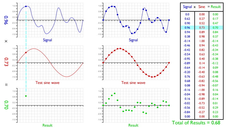
This total is the only result we need from our convolution operation. Once we’ve got the sum, we move onto the next harmonic sine wave and test that.

A few examples and some diagrams will make it clear.

Looking for the first harmonic in a ramp wave

First, let’s imagine we’re trying to determine the spectrum of a ramp wave. Not very realistic, since we can just look it up, but it’s a simple example.

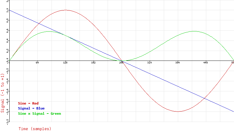
The blue line is the ramp signal under analysis.

Red is the sine signal (the 1st harmonic).

Green is the product of those two signals, one multiplied by the other.

Note that the green product is always positive. Consequently, the sum of all these samples is positive, and the area under the curve is positive, indicating that our waveform contains some amount of the first harmonic.

How would we actually code that? It’s pretty straight-forward:

// We have an input ‘signal’ array of ‘num_of_samples’ - the blue ramp wave
// We’ll test for the first harmonic in this example
$harmonic = 1;
$total = 0;                                    // This stores our output, the area under the green curve
for ($i=0; $i<$num_of_samples; $i++) {         // Loop through all the samples
    $sine_value = sin(2 * PI * $harmonic * $i / $num_of_samples);    // The red sine wave
    $product = $sine_value * $signal[$i];                            // The green curve
    $total = $total + $product;
}
// ‘total’ now contains the area under the curve generated by multiplying the signal by the sine harmonic.

And that’s basically it! There’s one more trick to come, but we’ll get to that later. Fourier analysis is composed of running the above code over and over, with different values of the ‘harmonic’ variable.

Since the sum will be larger if we have more samples, we need to divide by the number of samples to compensate and give us the same answer independent of whether we used a high sample rate or a low sample rate. So we should add:

$total = $total / $num_of_samples;

Since what we’v done is add up all the products and then divide by how many there were, we’ve taken the average (ok, ok, the “mean”) of all the products.

Looking for the first harmonic in a square wave

Ok, so let’s see the same thing with a square wave.

Again, the blue line is the square signal under analysis, the red is the sine signal (the 1st harmonic), and green is the product of those two signals.

Note that the green product is always positive here too. Consequently, the sum of all these samples must be positive, and the area under the curve is positive, indicating that our square waveform also contains some amount of the first harmonic.

Looking for the first harmonic in a DC signal

Ok, so what happens when the signal doesn’t have any of the harmonic we’re testing?

If we try and analyse a DC signal, we get a product (in green again) which is equally above and below the x-axis. The samples will sum to zero, and the positive and negative areas under the curve sum to zero.  My ‘total’ variable will end the loop with zero in, indicating that there’s no first harmonic in a DC signal!

Looking for the second harmonic in a square wave

Similarly, if we look for a second harmonic in a waveform that doesn’t include it, like a square wave, we get a zero result. You can clearly see that the positive and negative portions of the green curve are equal again.

Looking for the third harmonic in a square wave

If we next look for the third harmonic in the square wave, we get a result which is both positive and negative, but the majority of the result is positive, so the final total of the samples or the area under the curve is also positive.

This shows that the third harmonic is present in the square wave, albeit at a reduced level compared with the first harmonic.

By now, you should be starting to see how the simple multiplication and summing can give a measure of the amount of each harmonic in a waveform.

Incidentally, this “multiply and sum” is such an important  operation that in DSP land it usually gets its own instruction, MAC, for “multiply and accumulate”.

Working out the harmonic spectrum

Isn’t this great? We can work out the harmonic spectrum of any given waveform, just by doing some multiplication and adding. That’s pretty cool. Let’s expand our code a bit to test the first twenty harmonics:

// We have an input ‘signal’ array of ‘num_of_samples’ - the blue input wave
$num_of_harms = 20;       // We’ll create a ‘spectrum’ array of twenty harmonics in this example
$spectrum = array(20);    // Set up the array for the results
for ($h=1; $h<$num_of_harms+1; $h++) {       // Go through 20 harmonics
    $total = 0;                              // This stores our output, the area under the green curve
    for ($i=0; $i<$num_of_samples; $i++) {                     // Loop through all the samples
        $sine_value = sin(2 * PI * $h * $i / $num_of_samples); // The red sine wave
        $product = $sine_value * $signal[$i];                  // The green curve
        $total = $total + $product;
    }
    // ‘total’ now contains the area under the curve for this one harmonic
    $spectrum[$h] = $total / $num_of_samples;                  // Store this harmonic’s result
}
// Done! The spectrum array contains the amounts of all twenty harmonics

In truth, it isn’t quite this simple. One question is “What units are these harmonic levels measured in?”. Well, how big the output is depends on how big the input is, so it’s a relative measure. Typically, we’d regard the level of the highest harmonic as “1” and scale the others accordingly. To use the jargon, we “normalize” the amounts. Since the first harmonic is often (but by no means always) the largest, this often amounts to dividing the level of all the harmonics by the level of the first harmonic.

One further thing causes trouble – phase. So far we’ve been looking at nice, neat, clinical waveforms where all the harmonics start at phase zero. Most real-world waveforms are not this neat, although analog synths and signal generators produce waveforms that are.

What about phase?

What will happen if the signal includes a tested sine wave frequency, but that signal is out of phase with the sine wave we’re testing? Won’t this screw up the result?

Well, yes, it will. For example, let’s have another look a square wave and its first harmonic:

In this example, we’re testing the square wave with the same first harmonic as we used above, but this time the square wave is shifted by 90 degrees (128 samples on the diagram – same thing).  It’s a bit harder to see, but the result is that the green product is now equally above and below the line (two green half-lumps both up and down), and the total will sum to zero. Crikey! It doesn’t work any more! We broke it!

So how do we know whether we’ve got a small result because there’s only a small amount of the tested sine in the signal for analysis, or whether the result is small because the signal is partially out of phase?

The obvious way is to test the signal with sine waves at all the possible phases. The correct phase would give the largest result, enabling us to determine the phase as well as the amount.

In practice, it isn’t necessary to test every single phase to find the best result. The worst-case scenario in terms of phase is a 90-degree shift from our sine wave, like in the above example. At first glance, you might assume that a 180-degree shift would be the worst, but a 180-degree shift just gives us the same result as zero degrees of shift, except with the sign reversed. It’s the 90-degree shift that gives a zero result.

This gives us a clue to the solution. If we test with a sine wave and a 90-degree shifted sine wave, we have all the information we need to determine the phase. Since a 90-degree shifted sine wave is a cosine wave, we just test the signal with a sine wave and a cosine wave.

This is where the mathematicians start getting complicated about it. Instead of describing what they’re doing like this, they refer to this as a “complex frequency”, which is like a complex number, but with a sine wave and a cosine wave. The important part of that is that a sine and cosine wave differ by 90 degrees, just like the real and imaginary axes of a complex number (they’re “orthogonal”). However, there’s no need to start slinging terminology at the question. We just test with one, then the other, and then use a bit of simple trigonometry to get the phase.

Let’s update our code to include the cosine sum:

// We have an input ‘signal’ array of ‘num_of_samples’
// We’ll create a ‘spectrum’ array of twenty harmonics in this example
$num_of_harms = 20;
$spectrum = array($num_of_harms); // Set up the arrays for the results
$phases = array($num_of_harms);
for ($h=1; $h<$num_of_harms+1; $h++) { // Go through all the harmonics
    $sin_total = 0; // This time we test with both sine and cosine waves
    $cos_total = 0;
    for ($i=0; $i<$num_of_samples; $i++) { // Loop through all the samples
        // Test the signal with a sine wave
        $sine_value = sin(2 * PI * $h * $i / $num_of_samples);
        $sin_product = $sine_value * $signal[$i];
        $sin_total = $sin_total + $sin_product;
        // Test the same signal with a cosine wave too
        $cosine_value = cos(2 * PI * $h * $i / $num_of_samples);
        $cos_product = $cosine_value * $signal[$i];
        $cos_total = $cos_total + $cos_product;
    }
    // Get the mean (compensate for more or less samples)
    $sin_result = $sin_total / $num_of_samples;
    $cos_result = $cos_total / $num_of_samples;
    // Now we can work out the magnitude using Pythagoras' theorem
    $magnitude = sqrt(($sin_result * $sin_result) + ($cos_result * $cos_result));
    $spectrum[$h] = $magnitude; // Store this harmonic’s result
    // Now we can work out the phase using trigonometry
    if ($sin_result == 0) { // Avoid division by zero in the phase calculation
        $phase = M_PI / 2; // atan gives Pi/2 for infinite input
    } else {
        $phase = atan($cos_result / $sin_result);
    }
    $phases[$h] = $phase; // Store this harmonic’s result
}
// Done! The spectrum array contains the amounts of all twenty harmonics
// and the phases array contains the phases of those harmonics.

I hope this helps someone the way I would have liked it to have helped me when I was twelve.

Other useful stuff about the Fourier Transform on the web

Most of the articles I’ve seen on the web are as bad as the textbook stuff I was complaining about at the beginning of this article. However, here’s one that’s much better than that. Perhaps it can help the light come on for you.

BetterExplained.com: Fourier Transform

 

Update: Bug fix

My thanks to Stella Hall for spotting that I had the result wrong in the conditional that catches division by zero in the final code snippet. It previously said “$phase = M_PI”, but it should be “$phase = M_PI/2”. She also pointed out that in many languages, the atan2 function will avoid the need for the conditional statement, which simplifies this section to a single line:
$phase[$h] = atan2($cos_result, $sin_result);